Continuous Fourier Transform (non-periodic, continuous-time)

If you take the Fourier series and let the period $T \to \infty$, the discrete harmonic lines become continuous — resulting in the Continuous Fourier Transform (CFT). It represents general, non-periodic continuous-time signals.

CFT for a continuous sequence

$$X(f) = \int_{-\infty}^{\infty} x(t)\, e^{-j 2\pi f t} \, dt$$

Inverse CFT for a continuous sequence

$$x(t) = \int_{-\infty}^{\infty} X(f)\, e^{j 2\pi f t} \, df$$

note

• The CFT assumes a continuous-time signal $x(t)$ defined for all $t$.
• Not directly computable on a digital computer because it requires infinite, continuous data.
• The forward and inverse transforms differ in the sign of the complex exponential (which determines rotation direction) and—in discrete implementations—by a normalization factor (e.g. $\frac{1}{N}$ for the inverse DFT in the engineering convention). Both differences are required so the inverse undoes the forward transform.

---

Example: Gaussian pulse

A Gaussian pulse is a common non-periodic signal. Its CFT is also a Gaussian (frequency-domain spread inversely proportional to time-domain width). Note how the time-domain Gaussian width inversely affects the spread in the frequency domain in Figure 1.

In practice, we compute approximate transforms digitally using the DFT/FFT, which discretizes both time and frequency.

Figure 1: Gaussian pulse in time domain (top) and magnitude of its CFT (bottom)

You may have missed this

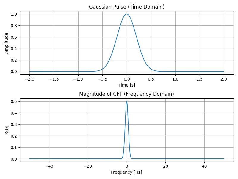
In previous sections, frequency-domain graphs showed the magnitude on the y-axis. Here, |X(f)| represents the same concept: the amplitude of each frequency component.

$|X(f)|$ is the same as what we referred to as "magnitude" in the previous sections.

View Figure 1's code

import numpy as np
import matplotlib.pyplot as plt

# Time vector
t = np.linspace(-2, 2, 1000)

# Gaussian pulse
sigma = 0.2
x_t = np.exp(-t**2 / (2*sigma**2))

# Frequency vector for plotting
f = np.linspace(-50, 50, 1000)

# Continuous Fourier Transform (analytical for Gaussian)
X_f = sigma * np.sqrt(2*np.pi) * np.exp(- (2*np.pi*f*sigma)**2 / 2)

# Plot
fig, axs = plt.subplots(2, 1, figsize=(8,6))

# Time domain
axs[0].plot(t, x_t)
axs[0].set_title("Gaussian Pulse (Time Domain)")
axs[0].set_xlabel("Time [s]")
axs[0].set_ylabel("Amplitude")
axs[0].grid(True)

# Frequency domain (magnitude)
axs[1].plot(f, np.abs(X_f))
axs[1].set_title("Magnitude of CFT (Frequency Domain)")
axs[1].set_xlabel("Frequency [Hz]")
axs[1].set_ylabel("|X(f)|")
axs[1].grid(True)

plt.tight_layout()
plt.show()