Fourier Series - the bridge (periodic signals)

The Fourier Series decomposes a periodic signal in the time domain into a sum of harmonics - sinusoidal components at integer multiples of the fundamental frequency. These harmonics represent the signal's building blocks in the frequency domain.

In other words, a periodic time-domain signal can be perfectly represented by adding together these harmonic sinusoids. Conversely, the Fourier series maps the time-domain periodic signal to discrete points in the frequency domain — its harmonic frequencies.

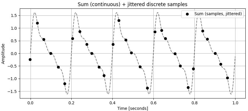
Figure 1: Sum Continuous (High-Resolution) with Actual Jittered Samples Overlaid

View Figure 1's Code

import numpy as np
import matplotlib.pyplot as plt

# === Parameters ===
f0 = 5
T = 1.0
Fs = 30
num_harmonics = 4
amplitudes = [1, 0.6, 0.35, 0.2]

# Time vectors
t_cont = np.linspace(0, T, 1000, endpoint=False)
t_disc = np.linspace(0, T, int(Fs*T), endpoint=False)
t_disc_jittered = t_disc + (np.random.rand(len(t_disc)) - 0.5) * (1/Fs) * 0.5

# Continuous sum
sum_cont = np.sum([A * np.sin(2*np.pi*k*f0*t_cont)
                   for k, A in enumerate(amplitudes, start=1)], axis=0)

# Jittered discrete sum
sum_disc_jittered = np.sum([A * np.sin(2*np.pi*k*f0*t_disc_jittered)
                            for k, A in enumerate(amplitudes, start=1)], axis=0)

# Plot
plt.figure(figsize=(10, 4))
plt.plot(t_disc_jittered, sum_disc_jittered, 'ko', label='Sum (samples, jittered)')
plt.plot(t_cont, sum_cont, 'k--', alpha=0.5)
plt.title("Sum (continuous) + jittered discrete samples")
plt.xlabel("Time [seconds]")
plt.ylabel("Amplitude")
plt.grid(True)
plt.legend()
plt.show()

Figure 1 (above) shows a periodic signal plotted over time with discretely sampled points.

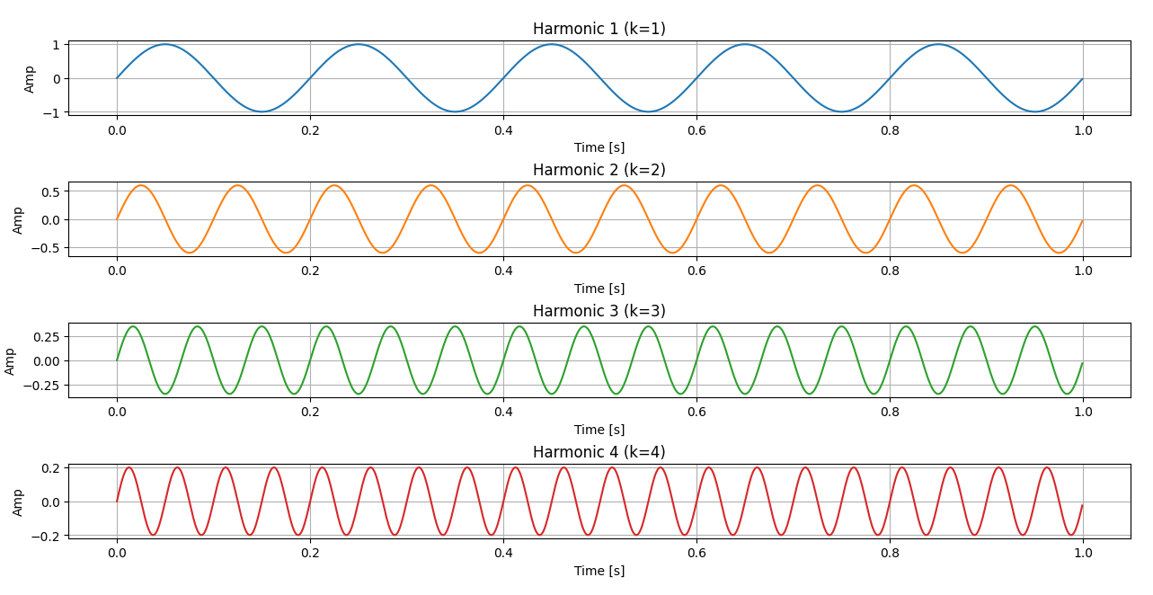
Figure 2 (below) illustrates each underlying harmonic as a continuous sine wave in the time domain.

Figure 2: Underlying Harmonics - Individual Continuous Harmonic Components

View Figure 2's Code

import numpy as np
import matplotlib.pyplot as plt

# === Parameters ===
f0 = 5
T = 1.0
amplitudes = [1, 0.6, 0.35, 0.2]

t_cont = np.linspace(0, T, 1000, endpoint=False)

# Individual harmonics
harmonics = [A * np.sin(2*np.pi*(i+1)*f0*t_cont) for i, A in enumerate(amplitudes)]

# Get the default color cycle from matplotlib
colors = plt.rcParams['axes.prop_cycle'].by_key()['color']

# Plot
fig, axs = plt.subplots(4, 1, figsize=(8, 10))  # 4 rows, 1 column
for i, ax in enumerate(axs):
    ax.plot(t_cont, harmonics[i], color=colors[i % len(colors)])
    ax.set_title(f"Harmonic {i+1} (k={i+1})")
    ax.set_xlabel("Time [s]")
    ax.set_ylabel("Amp")
    ax.grid(True)

plt.tight_layout()
plt.show()

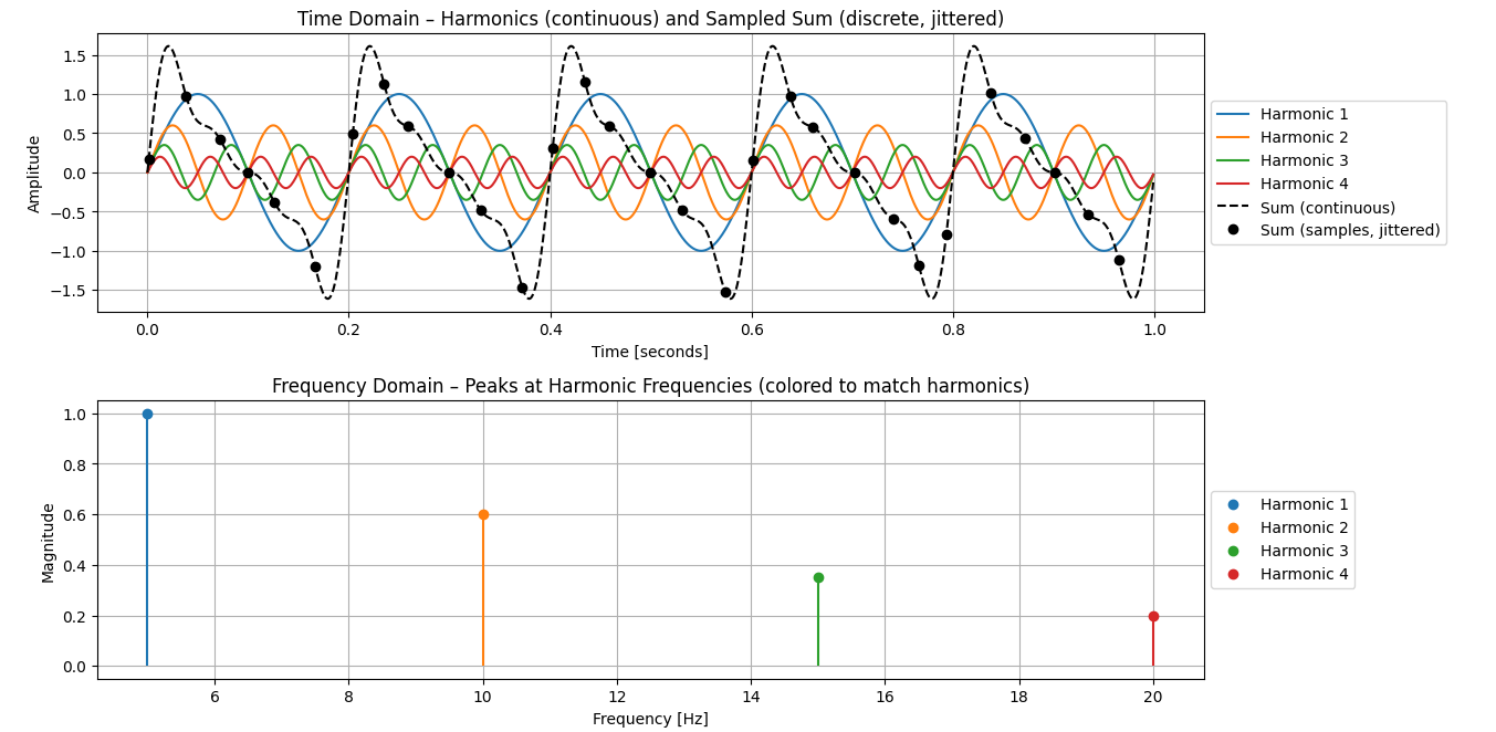
Figure 3: Combined Time-Domain Harmonics with Jittered Samples and Frequency Spectrum

View Figure 3's Code

import numpy as np
import matplotlib.pyplot as plt

# === Parameters ===
f0 = 5
T = 1.0
Fs = 30
amplitudes = [1, 0.6, 0.35, 0.2]

# Colors for harmonics
colors = ['C0', 'C1', 'C2', 'C3']  # matplotlib default color cycle

# Time vectors
t_cont = np.linspace(0, T, 1000, endpoint=False)
t_disc = np.linspace(0, T, int(Fs*T), endpoint=False)
t_disc_jittered = t_disc + (np.random.rand(len(t_disc)) - 0.5) * (1/Fs) * 0.5

# Harmonics and sums
harmonics = [A * np.sin(2*np.pi*(i+1)*f0*t_cont) for i, A in enumerate(amplitudes)]
sum_cont = np.sum(harmonics, axis=0)
sum_disc_jittered = np.sum([A * np.sin(2*np.pi*(i+1)*f0*t_disc_jittered)
                            for i, A in enumerate(amplitudes)], axis=0)

# Frequencies for Fourier peaks
freqs = np.array([f0*(i+1) for i in range(len(amplitudes))])

# --- Combined figure with subplots ---
fig, axs = plt.subplots(2, 1, figsize=(12, 8))

# Time domain plot
for i, harmonic in enumerate(harmonics):
    axs[0].plot(t_cont, harmonic, color=colors[i], label=f"Harmonic {i+1}")
axs[0].plot(t_cont, sum_cont, 'k--', label="Sum (continuous)")
axs[0].plot(t_disc_jittered, sum_disc_jittered, 'ko', label="Sum (samples, jittered)")
axs[0].set_title("Time Domain – Harmonics (continuous) and Sampled Sum (discrete, jittered)")
axs[0].set_xlabel("Time [seconds]")
axs[0].set_ylabel("Amplitude")
axs[0].grid(True)
axs[0].legend(loc='center left', bbox_to_anchor=(1, 0.5))  # legend outside the plot

# Frequency domain plot (colored)
lines = []
labels = []
for i, (freq, amp) in enumerate(zip(freqs, amplitudes)):
    markerline, stemlines, baseline = axs[1].stem([freq], [amp], linefmt=colors[i], markerfmt=f'{colors[i]}o', basefmt=" ")
    lines.append(markerline)
    labels.append(f"Harmonic {i+1}")

axs[1].set_title("Frequency Domain – Peaks at Harmonic Frequencies (colored to match harmonics)")
axs[1].set_xlabel("Frequency [Hz]")
axs[1].set_ylabel("Magnitude")
axs[1].grid(True)
axs[1].legend(lines, labels, loc='center left', bbox_to_anchor=(1, 0.5))  # legend outside the plot

plt.tight_layout()
plt.show()

Figure 3 (above) combines these harmonics (from figures 1 & 2) and shows the signal’s corresponding amplitude peaks at harmonic frequencies in the frequency domain.

The bottom panel in Figure 3 shows the frequency domain representation of the signal, highlighting discrete peaks at the harmonic frequencies corresponding to the sinusoidal components in the time domain.

Block Equation (Fourier Series)

A periodic signal $x(t)$ with period $T$ can be expressed as a sum of complex exponentials (or equivalently, sinusoids) at integer multiples of the fundamental frequency $f_0 = \frac{1}{T}$:

$$x(t) = \sum_{k=-\infty}^{\infty} X_k e^{j 2 \pi k f_0 t}, \quad \text{where } k \in \mathbb{Z} \text{, } X_k \in \mathbb{C}$$

• $k$ indexes the harmonics

  • e.g., $k=1$ is the first harmonic $(f_0)$, $k=2$ is the second harmonic $(2f_0)$, etc.

    • Hence $k f_0$ inside the exponent
    note

    $k=0$ corresponds to the DC component ($0 \text{ Hz}$), which is not considered a harmonic.

    $k < 0$ corresponds to negative frequency components (complex conjugates), which is important for understanding FFT symmetry.

• $X_k$ are the complex Fourier coefficients representing the amplitude and phase of each harmonic.
  • To interpret them:
    • Write $X_k = a + jb$ with $a = \Re(X_k)$ and $b = \Im(X_k), \quad \Re\text{: Real, } \Im\text{: Imaginary}$
    • Amplitude (magnitude): $|X_k| = \sqrt{a^2 + b^2} \quad \text{(Pythagoras)}$
    • Phase (angle): $\arg(X_k) = \tan^{-1}\left(\frac{b}{a}\right)$
  • This means the real part measures how much cosine of that frequency is present, the imaginary part measures how much sine, and together they define the sinusoid's amplitude and phase.

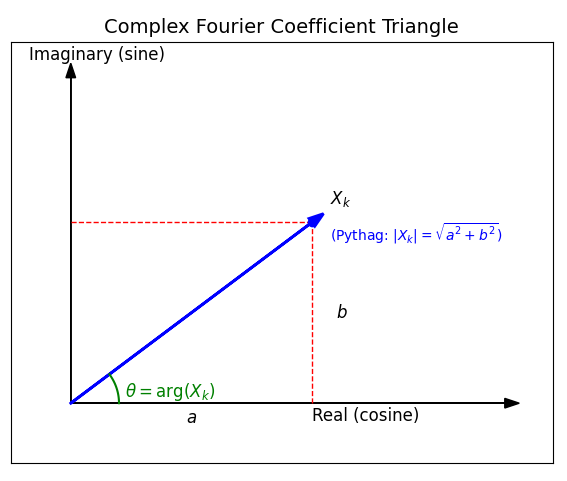
Understanding Magnitude and Phase of Fourier Coefficients

When you see a Fourier coefficient $X_k = a + jb$, it's easy to forget what the real and imaginary parts mean. Here's a clear way to visualize it:

Using Euler's formula ($e^{i \theta} = \cos\theta + i \sin\theta$), we know that:

• Real part ($a = \Re(X_k)$) → corresponds to the cosine component
• Imag part ($b = \Im(X_k)$) → corresponds to the sine component

Think of $X_k$ as a vector in the complex plane:

View the above image's code

import matplotlib.pyplot as plt
import numpy as np

# Fourier coefficient
a = 2.0   # Real part (cosine)
b = 1.5   # Imaginary part (sine)
c = np.sqrt(a**2 + b**2)
theta = np.arctan2(b, a)

# Plot setup
fig, ax = plt.subplots(figsize=(7,7))

# Draw axes with arrows
ax.arrow(0, 0, a*1.8, 0, head_width=0.08, head_length=0.12, fc='black', ec='black')
ax.arrow(0, 0, 0, b*1.8, head_width=0.08, head_length=0.12, fc='black', ec='black')

# Draw vector X_k
ax.arrow(0, 0, a, b, head_width=0.08, head_length=0.12, fc='blue', ec='blue', linewidth=2)

# Draw dashed triangle sides
ax.plot([a, a], [0, b], color='red', linestyle='--', linewidth=1)
ax.plot([0, a], [b, b], color='red', linestyle='--', linewidth=1)

# Annotations - outside the triangle
ax.text(a/2, -0.05, r'$a$', fontsize=12, ha='center', va='top')                     # Real side
ax.text(a + 0.2, b/2, r'$b$', fontsize=12, ha='left', va='center')                   # Imag side

# Phase angle arc
arc = np.linspace(0, theta, 50)
arc_radius = 0.4
ax.plot(arc_radius*np.cos(arc), arc_radius*np.sin(arc), color='green', linewidth=1.5)
ax.text(0.45, 0.05, r'$\theta = \arg(X_k)$', fontsize=12, color='green')

# Vector tip label
ax.plot(a, b, 'o', color='blue')
ax.text(a + 0.15, b + 0.15, r'$X_k$', fontsize=12)
ax.text(a + 0.15, b + -0.15, r'$(\text{Pythag: } |X_k| = \sqrt{a^2 + b^2})$', fontsize=10, color='blue')  # Note

# Axes labels - moved to avoid overlap
ax.text(a, -0.15, 'Real (cosine)', fontsize=12)
ax.text(-0.35, b*1.9, 'Imaginary (sine)', fontsize=12)  # moved up

# Set limits and aspect
ax.set_xlim(-0.5, a*2)
ax.set_ylim(-0.5, b*2)
ax.set_aspect('equal', 'box')

# Remove ticks
ax.set_xticks([])
ax.set_yticks([])

# Title
ax.set_title('Complex Fourier Coefficient Triangle', fontsize=14)

plt.show()

Key points:

1. Amplitude (magnitude): $$|X_k| = \sqrt{a^2 + b^2}$$ This is the hypotenuse of the triangle and gives the overall strength of the sinusoid.
2. Phase (angle): $$\arg(X_k) = \theta = \tan^{-1}\left(\frac{b}{a}\right)$$ This is the angle the vector makes with the real axis — the phase shift of the sinusoid.
3. Trigonometric intuition: Using SOH CAH TOA:
   • Opposite side → $b$ (imaginary / sine)
   • Adjacent side → $a$ (real / cosine)
   • $\tan\theta = \frac{b}{a}$ → angle of the vector

Why this matters:

The real and imaginary parts tell you how much cosine and sine of that frequency are in the signal. Combining them using Pythagoras gives the amplitude, and the angle gives the phase, which shifts the waveform in time. This is exactly how $X_k$ encodes both strength and timing of each harmonic.

• $f_0 = 1/T$ is the fundamental frequency, the lowest frequency of the periodic signal.

Intuition

Every periodic signal can be “built” by adding together these harmonics. The series tells us exactly how much of each harmonic is present.

Real Fourier Series Form

The Fourier series can also be expressed using only real-valued sine and cosine functions:

$$x(t) = a_0 + \sum_{k=1}^{\infty} [ a_k \cos(2 \pi k f_0 t) + b_k \sin(2 \pi k f_0 t) ]$$

• $a_0$ is the DC component (average value of the signal).
• $a_k$ and $b_k$ are the real Fourier coefficients representing the amplitudes of cosine and sine components at the $k^\text{th}$ harmonic.
• This form is equivalent to the complex exponential form: $$X_k = \frac{1}{2}(a_k - j b_k), \quad X_{-k} = \frac{1}{2}(a_k + j b_k)$$ so the information about amplitude and phase is fully captured.

Fourier Coefficients (Complex Amplitudes)

The coefficients $X_k$ quantify the contribution of each harmonic $k$ in the signal:

$$X_k = \frac{1}{T} \int_{0}^{T} x(t) \cdot e^{-j 2 \pi k f_0 t} dt$$

• This integral measures how much of the frequency $k f_0$ exists in the signal.
• You can integrate over any interval of length $T$, because the signal is periodic.
• In practice:
  • $|X_k|$ gives the amplitude of the $k^\text{th}$ harmonic.
  • $\arg(X_k)$ gives its phase (how much it’s shifted in time).

Visual analogy

Imagine projecting your signal onto each sine/cosine component — the integral tells you the “shadow” of the signal along that harmonic.

tip

$a_k$ and $b_k$ can be converted to amplitude and phase using:

$$\begin{align*} A_k &= \sqrt{a_k^2 + b_k^2}\\ \phi_k &= \tan^{-1}(\frac{ b_k }{ a_k }) \end{align*}$$