Introduction

Fourier techniques let us express any signal as a sum of its constituent "pure" sinusoids (frequencies), meaning:

• "Pure" sinusoids: any signal is composed of simple sinusoids, e.g.:

$$\sin(2\pi f_1 t),\quad \sin(2\pi f_2 t)$$

• Sum of constituent frequencies: any signal equals the sum of its "pure" constituent sinusoids, e.g:

$$x(t)=\sin(2\pi f_1 t)+\sin(2\pi f_2 t)$$

This gives two equivalent ways of describing a signal:

• Time domain — how the signal changes over time
• Frequency domain — how much of each frequency is present

The Fourier Transform converts between these representations.

Sinusoids

Continuous Sinusoids

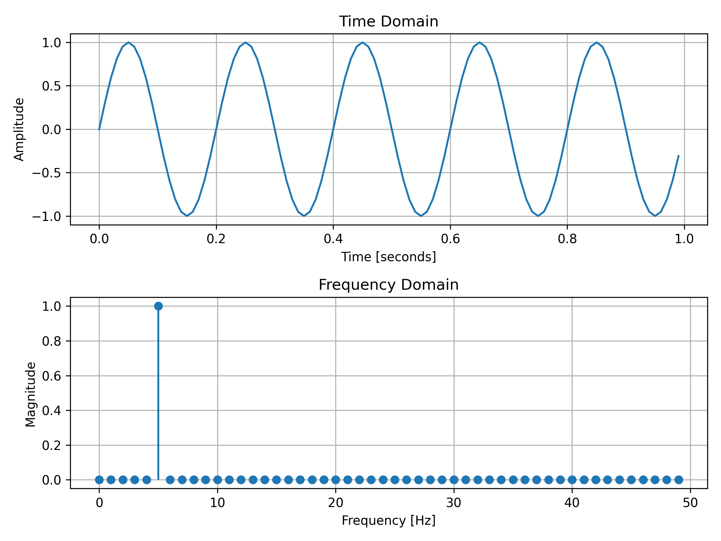
For the purpose of illustration, we’ll treat the finely sampled sinusoid in Figure 1 as a continuous signal.

Below, Figure 1 shows the exact same sinusoid plotted in both the time and frequency domain. Notice how the time domain graph looks like the typical wave shape of a sine graph that you are likely familiar with, whereas the frequency domain graph contains only one non-zero point, $(5, 1)$. This is because the signal contains only a single pure tone (see f0 in Figure 1's Python Code).

info

Continuous sinusoidal data are best-suited for CFTs (Continuous Fourier Transforms).

Figure 1: A densely sampled sinusoid to approximate a continuous signal plotted in time and frequency domains

View Figure 1's Code

import numpy as np
import matplotlib.pyplot as plt

# === Parameters ===
f0 = 5          # Frequency of the sinusoid in Hertz (cycles per second)
fs = 100        # Sampling frequency in Hertz (how many samples per second)
duration = 1    # Duration of the signal in seconds

# === Time vector and signal ===
# Create an array 't' of evenly spaced time points from 0 up to (but not including) 1 second.
# The total number of points = fs * duration = 100 samples.
t = np.linspace(0, duration, int(fs * duration), endpoint=False)

# Generate the sinusoidal signal:
# x(t) = sin(2 * π * f0 * t)
# Explanation:
# - '2 * π * f0' converts frequency in Hz to angular frequency in radians per second.
# - 'sin()' takes the angle in radians.
x = np.sin(2 * np.pi * f0 * t)

# === Fourier Transform ===
# Compute the Fast Fourier Transform (FFT) of the signal to get its frequency components.
X = np.fft.fft(x)

# Get the corresponding frequencies for each FFT bin.
# The 'fftfreq' function returns frequencies from 0 up to positive Nyquist frequency,
# then negative frequencies after that.
freqs = np.fft.fftfreq(len(X), 1 / fs)

# We only need the positive half of the frequencies and magnitudes since
# the FFT of a real-valued signal is symmetric.
positive_freqs = freqs[:len(freqs) // 2]

# Magnitude of the FFT (absolute value) normalized by half the length of X.
# This scaling ensures the amplitude matches the original sinusoid amplitude.
magnitude = np.abs(X)[:len(freqs) // 2] / (len(X) / 2)

# === Plotting ===
fig, (ax1, ax2) = plt.subplots(2, 1, figsize=(8, 6))

# Time domain plot: signal amplitude vs time
ax1.plot(t, x)
ax1.set_title("Time Domain")
ax1.set_xlabel("Time [seconds]")
ax1.set_ylabel("Amplitude")
ax1.grid(True)

# Frequency domain plot: magnitude of frequency components vs frequency
ax2.stem(positive_freqs, magnitude, basefmt=" ")
ax2.set_title("Frequency Domain")
ax2.set_xlabel("Frequency [Hz]")
ax2.set_ylabel("Magnitude")
ax2.grid(True)

plt.tight_layout()

# Uncomment this line to save the figure as a PNG image file:
# plt.savefig("continuous-sinusoid.png", dpi=300)

plt.show()

Discrete Sinusoids

In this repo we operate on digital data (images/arrays), which are sampled, finite, and stored in memory since real digital systems (microcontrollers, sensors, images) cannot store continuous signals. They store samples, collected at discrete time intervals.

That makes the DFT the natural mathematical tool that we will use since we do not have continuous data (our data came from samples taken at intervals - random or constant). The DFT converts a finite (discrete) sequence of samples into a set of frequency-domain coefficients that we can filter, manipulate (e.g. by multiplying by frequency-domain kernels in a Gaussian blur), and then convert back to the time domain.

info

Discrete sinusoidal data are best-suited for DFTs (Discrete Fourier Transforms).

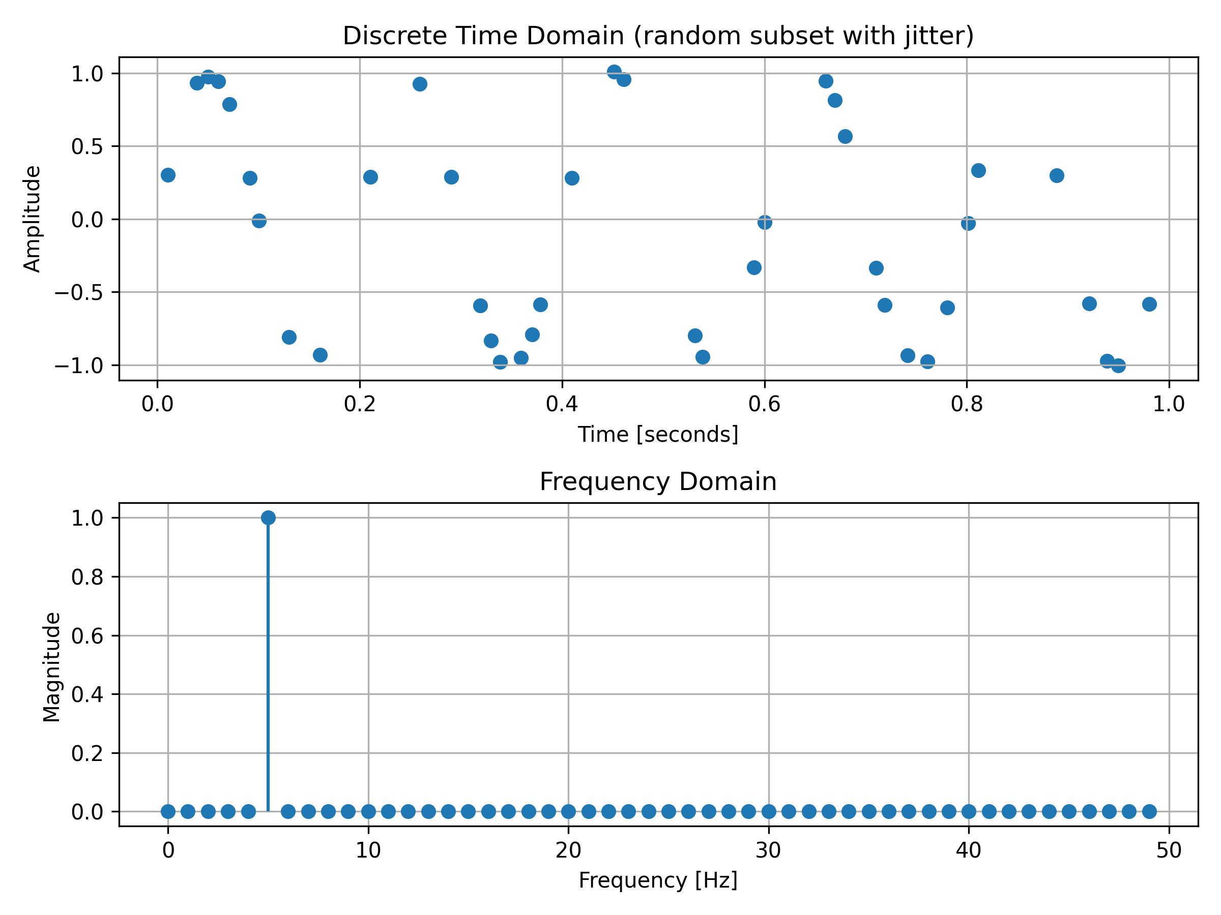
Figure 2: A realistically sampled sinusoid plotted in time and frequency domains

View Figure 2's Code

import numpy as np
import matplotlib.pyplot as plt

# === Parameters ===
f0 = 5          # Frequency of the sinusoid in Hertz (cycles per second)
fs = 100        # Sampling frequency in Hertz (samples per second)
duration = 1    # Duration of the signal in seconds

# === Discrete time vector and signal ===
# Number of samples = sampling frequency * duration
N = int(fs * duration)

# Create an array 'n' of discrete time indices from 0 to N-1
n = np.arange(N)

# Generate the discrete-time sinusoidal signal:
# x[n] = sin(2 * π * f0 * n / fs)
# Explanation:
# - 'n / fs' converts discrete index to actual time in seconds.
# - '2 * π * f0' converts frequency in Hz to angular frequency.
x = np.sin(2 * np.pi * f0 * n / fs)

# === Choose a random subset of points for plotting (fewer, but not too few) ===
# num_points: how many dots to show on the time plot
num_points = 40
# Safety clamp in case N < num_points
num_points = min(max(1, num_points), N)

# Randomly pick indices WITHOUT replacement, then sort them so points progress left-to-right
chosen_indices = np.sort(np.random.choice(n, size=num_points, replace=False))
n_down = chosen_indices
x_down = x[n_down]

# Add small random jitter:
# x_jitter_frac: fraction of the sample interval (1/fs). 0.15 => ┬▒15% of sample interval horizontally.
# y_jitter: absolute amplitude jitter (in signal units). Keep small so the waveform is still visible.
x_jitter_frac = 0.15
y_jitter = 0.03

x_jitter = (np.random.rand(len(n_down)) - 0.5) * (1 / fs) * 2 * x_jitter_frac
y_jitter = (np.random.rand(len(n_down)) - 0.5) * 2 * y_jitter

# === Fourier Transform ===
# Compute the Discrete Fourier Transform (DFT) using FFT to get frequency components.
X = np.fft.fft(x)

# Get the corresponding frequencies for each FFT bin.
# The 'fftfreq' function returns frequencies from 0 up to positive Nyquist frequency,
# then negative frequencies after that.
freqs = np.fft.fftfreq(N, 1 / fs)

# We only need the positive half of the frequencies and magnitudes since
# the FFT of a real-valued signal is symmetric.
positive_freqs = freqs[:N // 2]

# Magnitude of the FFT (absolute value) normalized by half the length of X.
# This scaling ensures the amplitude matches the original sinusoid amplitude.
magnitude = np.abs(X)[:N // 2] / (N / 2)

# === Plotting ===
fig, (ax1, ax2) = plt.subplots(2, 1, figsize=(8, 6))

# Time domain plot: discrete dots (fewer), with jitter, no connecting lines
ax1.scatter(n_down / fs + x_jitter, x_down + y_jitter, marker='o')
ax1.set_title("Discrete Time Domain (random subset with jitter)")
ax1.set_xlabel("Time [seconds]")
ax1.set_ylabel("Amplitude")
ax1.grid(True)

# Frequency domain plot: magnitude of frequency components vs frequency
ax2.stem(positive_freqs, magnitude, basefmt=" ")
ax2.set_title("Frequency Domain")
ax2.set_xlabel("Frequency [Hz]")
ax2.set_ylabel("Magnitude")
ax2.grid(True)

plt.tight_layout()

# Uncomment this line to save the figure as a PNG image file:
# plt.savefig("discrete-sinusoid.png", dpi=300)

plt.show()

Notice, once again, how the time domain graph looks like the typical wave shape of a sine graph that you are likely familiar with (even if it is a bit broken up due to poorly-timed sampling), whereas the frequency domain graph contains only one non-zero point, $(5, 1)$. This is because the signal contains only a single pure tone (see f0 in Figure 2's Python Code above).

Realistic Sinusoids

Figure 1 shows the ideal scenario: a clean sinusoid sampled densely enough to look continuous.

Figure 2 shows the type of data we actually work with in real programs: discrete, finite samples.

Both figures (1 and 2) represent the same sinusoid:

$$x(t)=\sin(2\pi f_0 t), \quad f_0=5 Hz$$

This distinction is the entire reason the DFT exists.

Above, Figure 2 is more representative of the data we are likely to encounter since the sensors we use measure data at imprecise intervals (due to slight natural variations) rather than continuously - it wouldn't be possible to get a continuous reading from them. Hence, DFTs are better suited for the domain conversions in this context.

Why use an FFT over a DFT or a CFT?

In practice, we only deal with two major Fourier transforms:

• the Continuous Fourier Transform (CFT)
• the Discrete Fourier Transform (DFT)

The Fast Fourier Transform (FFT) is not a different kind of transform - it's just a faster way to compute the DFT.

FFT = "DFT's practical implementation"

The FFT is just a fast algorithm for computing the DFT: they are mathematically identical. The only reason FFTs appear everywhere is because they are essentially just fast DFTs:

• DFT = mathematical definition
• FFT = optimized algorithm that computes a DFT

In computation, all data are discrete and finite, so only the DFT (via FFT) matters.

Fourier Transforms

Why use them?

Images, audio, and signals are discrete. Any filtering or transformation done in the frequency domain operates on discrete data, and must therefore use the DFT (via FFT). This is the foundation for FFT-based convolution, image kernels, Gaussian blurs, etc.

Why not use something simpler to understand?

Fourier Transforms can be avoided, but avoiding them often results in more significant drawbacks - motivating their use.

Time Complexity

One of the most important concerns about not using them is the resultant time complexity of functions.

Discussing all of the drawbacks is out of scope for this documentation, but it is worth mentioning one for the sake of your understanding:

Gaussian blurs on user-selected images

info

This is important because it covers one of the core processing techniques used in Img2Num's pre-processing pipeline before images are sent through K-means clustering.

Gaussian blur is a convolution of an image with a Gaussian kernel (window). For an image of size $N \times N$ and a kernel of size $K \times K$, direct convolution has a complexity of $O(N^2 K^2)$, but because Gaussian kernels are separable, it can be reduced to two 1D convolutions - horizontal and vertical - giving $O(N^2 K)$

This means the runtime scales linearly with the kernel size.

Using the FFT, convolution can be done in the frequency domain:

Action	Time Complexity
Compute FFTs of image & kernel	$O(N^2 \log N)$
Multiply FFTs of image & kernel	$O(N^2)$
Perform inverse FFT of image	$O(N^2 \log N)$
Total (independent of kernel size)	$O(N^2 \log N)$

FFT-based convolution is preferred for large kernels or images, where direct convolution becomes slow, while separable convolution is usually faster for small kernels due to lower overhead.

note

For extremely small kernels, direct or separable convolution may still be faster due to lower overhead.

Consider a $512 \times 512$ image with a small Gaussian kernel, say $5 \times 5$.

• Direct separable convolution: $O(N^2 K) = 512^2 \cdot 5 \approx 1.31 \times 10^6$ operations.
• FFT-based convolution: $O(N^2 \log N) = 512^2 \cdot \log_2 512 \approx 3.84 \times 10^6$ operations.

Here, direct convolution is ~3× faster because the kernel is small and the FFT overhead dominates.

This is, however, rarely the case for Img2Num's Gaussian blur since users are unlikely to upload such small images and the benefit of using an FFT is evident when a large image is uploaded.